A short message to the reader:

A genetic algorithm minimization is excellent to scan quickly the configuration space!

Introduction

A common way of treating experimental data is to fit them using a matematical model, the parameters of which have particular physical meaning. The key issue in this case is to select an appropriate model for the event measured and the measuring method employed and to use reliable fitting algorithms. Often, mainly in the case of problems which many degrees of freedom, the classical minimizig methods are difficult to use even when the model is appropriate. The reason is the difficulty to find a good starting set of parameters on which the success of these methods usually strongly depends. To estimate these parameters all possible apriori information must be used. Often, only intervals where where the respective values lie, are available. The knowledge of only the orders of respective values is usually not sufficient to estimate good strating parameters. Similar situation is met when the matematical model does not cover the full physical reality and complexity but it a reasonable simplification. In these situations, according to our experience, the use of genetic algorithm (GA)[1] is fruitful. It is so because for this method the estimation of parameters in a form of their margins is natural and it is less prone to end up in a local minima.

It has to be stressed that the GA method is not effective to make a fit "all the way" but it is exellent to find a good starting set of parameters which can further be used by standard minimizing methods.

First we describe the principle of the GA method and its connection with fmins, standard minimizing method intrinsic in Matlab. Later we illustrate the usefulness of our method by three typical examples from our practise[2].
 

The Method of Genetic Algorithm and Notes on the Fuction Programmed in Matlab

The GA method is based on coding the fitted parameters into a bit string. In each iteration a whole set of these strings, called the generation, is processed. Each member of a generation, which represents a particullar tentative set of parameters, is used to evaluate the trial function. The quality of fit of experimental data is found using a certain criteria. Then strings are ordered according to their success in fiting. The best are then taken as parents and are combined (crossed) to create a new generation. By this procedure good properties foor the fit are inherited. To avoid a falling into a trap of local minima a mutation process, based on random change of a small number of bits in a generation, introduced. This causes a jump into a different region of the configurational space. In the next iteration it is tested whether the jump was justified. If not the calculation is returned to the original point.

The main advantage of the GA method is its relative insensitivity to the selection of the starting set of parameters. This selection is made in the process of coding, where each parameter is given a certain interval of values and e certain precission. These properties then imply the length of the bit string and thereby one size of the configuration space. The other size is given by the number of parents and so the number of children in the next generation.

The main properties of the GA were thoroughly tested both on simulated and experimental data from several fields. It has been found that the process of inheritage of good properties and jumps in the configurational space leads quite fast relatively close to the accurate values of the parameters. Further precising of the parameters is, however, problematic since the process of inheritage ceases to be effective after several itterations and the random mutations which become the only tool for improvement, are in fact disturbing the minimization. The probability that a jump into a different region of the configuration space will mean an improovement is decreasing in the course of the calculation. Possible, yet complicated improvement of the GA method could use the fact of inequal weight of various bits representing parameters i a special smart mutations routine. Fortunately, it
turns out that the parameters obtained in a relative short time are usually a good starting set for further minimization by more standard techniques.

The Matlab turns out to be suitable to be used by our method. It is due to its ability to deal with whole matrices and availibility of other convenient intrisic functions. For instance most of the operatios on the whole generation can be performed at once and the comparison of the trial function and the experimental data can be accomplished by one command (this is the slowest part of the calculation). All matrices contain zeros and ones. Binary aritmetic is not employed (does it exist?)  .

Our routine is quite general and the precision of results can be traded for the speed of calculations. Since our objective is not the final minimization with the highest possible precision, we code each parameters by 8 bits only. The precision is still 0.4% of the span, which is usually sufficient. The advantage of this is a reasonable length of the bit strings.

We use two sexes and number of parents which cross in each generation can be selected by a parameter. Each of np  mothers has exactly one offspring with each of the np fathers and bits inherited from each of the parents are chosen randomly in each crossing. During the development of our method we tryied to use more then two sexes. It had shown up, however, that this brought only a computational cost and the same effect can be reached with two sexes and sufficient number of parents and thereby offsprings in each generation. This is in accord with the existence of two sexes in the nature.

Particularly the crossing can be accomplished easily using matrix arithmetic. First the matrix of mothers is prepared. The multiplicity of each mother is equal to the np. First column is the first mother, second is the second mother and np th column is the last mother. This pattern of columns is repeated np times. Similarly the matrix of fathers is created but here the first np colums are the first father the next np columns are the second father etc. Now two disjunct matrices, the sum of which is a matrix containing ones, are prepared. They control which bit is inherited from which parent. The mother matrix is (dot) multiplied by the first filter matrix the fathers matrix is multiplied by the second and the results are added giving the next generation of offsprings.

Mutations are controled by another matrix. It contains zeros except at the places where bits in the generation matrix will be toggled. The density of ones, usually very low, ic controled by a single parameter and their possitions are random. This mechanism doesn't take into account that the significance of bits so the size of the jump in the configurational space depends on which bit is particularly toggled. In our case we let the jumps be deliberately large. When the jump makes the fit worse, the calculation is not returned into the situation before jump but the best fits are remembered.
 
The resulting routine is universa for most problems. Its parameters are the mane of the function to be fitted, the matrix of searched parameters spans and computation parameters matrix. The last controls for instance number of parents, number of itterations, the measure of mutations and condition for plotting of the intermediate results. The function it self takes care for appropriate coding and performs the minimization with particular lenght and number of bit strings. After performing the desired number of itterations the routine returns the best fit, it has found.
 

The GA routine is followed by minimization using the function fmins, intrinsic to the Matlab. It uses the best values gained by the GA routine as its starting parameters.
 

Ilustrations of the combined method

We are showing the use of our method on three examples. The first two are from the field of time-resolved SAXS data treatment, the third concerns fitting of reflectivity data in solid-state physics.

SAXS data generally contain information on the size, shape and internal structure of inhomogenities of scattering density, which have, so called, colloid dimension. Particularly in the case of time-resolved measurements is the background physics too complicated to be expressed by a single model. Moreover the quality of data is low and it decreases with the desired time resolution. The usual data treatment methods divide the problem into steps. Usually some differential and integral parameters are calculated for every curve (frame or time-slice) and then their development in time is drawn.

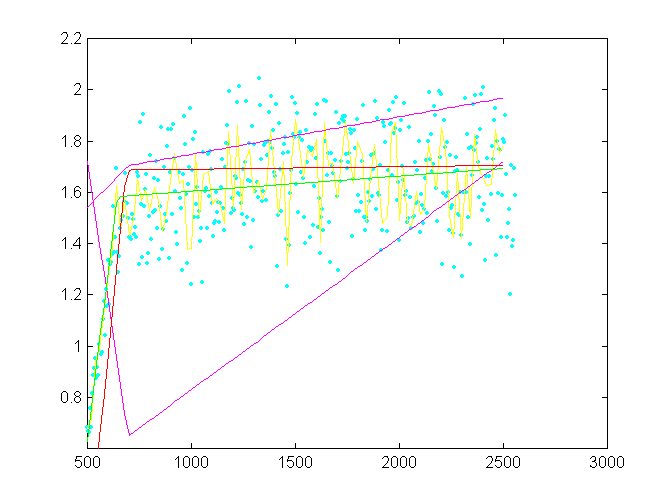
In the fig. 1 time development of the square of the scattering density of the amorphous and crystalline phase data are depicted. These quntities are the results of ratio of another experimental dependences and their quality is very low. It is anyway possible to see, without going into details, that the process of crystallization apparently proceeds in two stages differing in the speed. To characterize them more precisely data could be fitted by bilinear function. Due to the poor quality of data this is very difficult by standard methods. The GA on the other hand gives only after a few itterations a fit which doesn't describe the behaviour accurately but the parameters are a good starting set for the next minimization.  

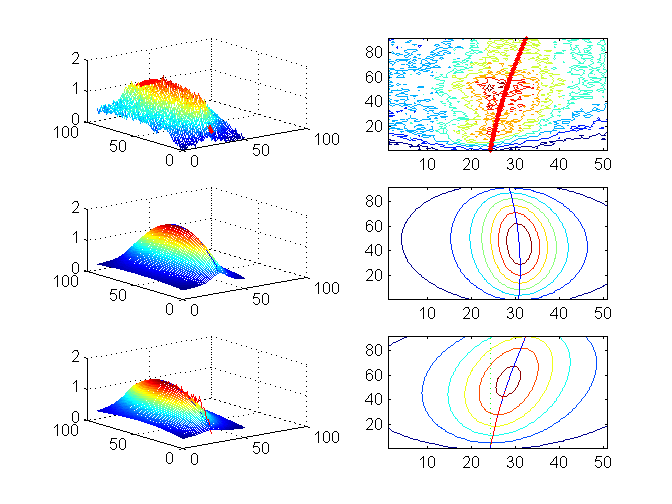
In the fig. 2 two dimensional fit directly from experimental data of time resolved SAXS data is shown. The properties of one peak is parametrized (not appropriatelly) by Lorentz function. If a region, where only one peak exists, is taken itno accont, the time development can be approximated by equation

Here p₁ is a constant background,   p₂, p₃, p₄ describes parabolic (in time) behaviour of the height of the peak,  p₅, p₆, p₇ parabolic behaviour of the position and  p₈, p₉ linear beahviour of the width. Of these parameters, particularly those describing the movement of the position of the peak have apparent meaning and can be a source of physically interesting information on interplane distances in the crystallic structure. The interpretation of the other parameters concerning the height and width is more complicated but these hold information on the quality of the order.

Due to the number and low transparency of these parameters a reliable estimation of the good starting parameters is next to impossible. Again, our method gives fair yet not exact impression on the behaviour of the peak.
 

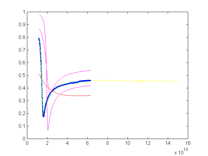
Last ilustation in the fig. 3 shows a fit of reflectivity data. Here a reasonable model using four parameters exists. Their values span, however,  several orders and their effect in the data is complicated and by no means transparent. Again, it is almost impossible to estimate a good set of starting parameters. The GA method reliable finds this set in spite of the fact that the apriory information is only on orders of the parameters.
 
 

Conclusion

A minimizing method has been developed which is based on calculating the starting set of parameters using the genetic algorithm method and then passing them to a standard fitting function. This method prooves to be efficient in cases when it is difficult to find this set reliably and easily but the span of values for each parameter can be estimated. This efficiency is illustrated on three typical examples.
 

In this place we would like to thank the Grant Agency of the CR for the support in the frame of the grant 109/99/0557.
 
 

[1] D. E. Goldberg, "Genetic Alghoritms in Search, Optimisation and Machine Learning", Adison-Wesley, Reading, MA. (1989)

[2] M. Steinhart, M.Kriechbaum, M. Horký, J. Baldrian, H. Amenitsch, P. Laggner and S. Bernstorff, "Time-resolved SAXS measurements of effects induced by variation of pressure", Materials Structure in Chemistry, Biology, Physics and Technology, in press
 
 
 
 

Fig.1:  A fit of bilinear function on time resolved SAXS data. Blue points are experimental data. Yellow dar data smoothed by splines. Smoothing in not necessary but it shortens the calculations since it reduces number of data. The difference in parameters is insignificant. The estimations in various itterations of the GA methos are violet and the best GA fit is red. These parameters are used for further minimization by fmins whose results are green. The GA method here uses 14 pairs of parents (np), 10 itterations and large mutations. The reproducibility is in three digits.
 
 
 
 

Fig. 3.: A fit of a reflectivity measurement. Experimental data are yellow. Blue points show the selected region. GA trials are magenta and the best GA fot is red. The final fit is green. The GA conditions are the same as in the previous case.
 
 
 
 

Fig. 2: Two-dimensional fit of time-resolved SAXS data. On the left side three-dimensional plots of intensities and in the right side their projection into the angle time plane are shown. In the first line raw data with the red final fit showing the developnemt of the position of the peak is depicted. In the second line output from the GA method and in the third line the final fit are shown. In the projections the development in-time of the peak position is hinted.
 
 

Contact address: stein@imc.cas.cz